Page 187 - The Geological Interpretation of Well Logs

- THE DIPMETER -

DIP PLOT DIP AZIMUTH STICK PLOTS
O° 90° 360°/0° 180° 90° _270°

— =
1950 = =
—
«
=|
= =
rs a | =
- 7 =|5
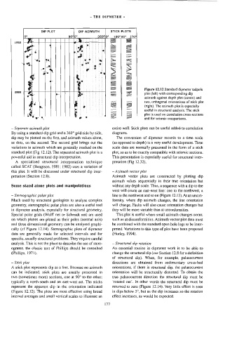
nef SS ES Figure 12.12 Standard dipmeter tadpole
>
-”
ye
=P
=
——
e
ws
==
=
=

=
=

=
2000
=
plot (left) with corresponding dip
.

azimuth against depth plot (centre) and
—
2 i
=
two, orthogonal orientations of stick plot
=
|
useful in structural analysis. The stick
—
=
=>
plot is used on correlation cross-sections
ji
and for seismic comparisons.
. & i | 2 oe? a = (right). The azimuth plot is especially
=
a
— Separate azimuth plot entire well. Stick plots can be useful added to correlation
By using a standard dip grid and a 360° grid side by side, diagrams.
dip may be plotted on the first, and azimuth values alone, The conversion of dipmeter records to a time scale
as dots, on the second. The second grid brings out the (as opposed to depth) is a very useful development. Time
variations in azimuth which are generally masked on the scale data are normally presented in the form of a stick
standard plot (Fig 12.12). The separated azimuth plot is a plot, so as to be exactly compatible with seismic sections.
powerful aid in structural dip interpretation. This presentation is especially useful for structural inter-
A specialised structural interpretation technique pretation (Fig 12.32).
called SCAT (Bengtson, 1981; 1982) uses a variation of
this plot. It will be discussed under structural dip inter- — Azimuth vector plot
pretation (Section 12.8). Azimuth vector plots are constructed by plotting dip
azimuth values sequentially in their true orientation but
Some stand alone plots and manipulations without any depth scale. Thus, a sequence with a dip to the
west will create an east-west line: one to the northwest, a
— Stereographic polar plot line to the northwest and so on (Figure 12.13). At an uncon-
Much used by structural geologists to analyse complex formity, where dip azimuth changes, the line orientation
geometry, stereographic polar plots are also a useful tool will change. Faults will also cause orientation changes but
in dipmeter analysis, especially for structural geometry. they will be more variable than at unconfonnities.
Special polar grids (Wulff net or Schmidt net} are used This plot is useful where small azimuth changes occur,
on which planes are ploted as their poles (normal axis) such as at disconformities. Azimuth vector plot data must
and three dimensional geometry can be analysed graphi- be combined with the standard open hole logs to be inter-
cally (cf Figure 12.14). Stereographic plots of dipmeter preted. Variations to this type of plot have been proposed
data are generally made for selected intervals and for (Hurley, 1994).
specific, usually structural problems. They require careful
analysis. This is not the place to describe the use of stere- — Structural dip rotation
ogcams, the classic text of Phillips should be consulted An essential routine in dipmeter work is to be able to
(Phillips, 1971). change the structural dip (see Section 12.8 for a definition
of structural dip). When, for example, palaeocurrent
— Stick plot directions are obtained from sedimentary cross-bed
A stick plot represents dip as a line. Because no azimuth orientations, if there is structural dip, the palaeocurrent
can be indicated, stick plots are usually presented in orientation will be structurally distorted. To obtain the
two (sometimes more) sections, one at 90° to the other: true palaeocurrent direction the structural dip must be
typically a north-south and an east-west set. The sticks ‘rotated out’. In other words the structural dip must be
represent the apparent dip in the orientation indicated returned to zero (Figure 12.14). Very little effect is seen
(Figure 12.12). The plots are most effective using broad in dips below 5°, but as the dip increases so the rotation
interval averages and small vertical scales to illustrate an 177 effect increases, as would be expected.