Page 221 - The Geological Interpretation of Well Logs

- IMAGE LOGS -

coal
roots

foresets 4
est N
29.15.01) RQXX¥V | Fig. 13.16 Zz

ANS foresete =
“ f=
“Se
IS)
2950.0 |
érosion
finely laminated

2955.0
c
clay plug
iw

—s =
2960.0 KYAAA forasete <
|
| | Sesh G

erosion
\
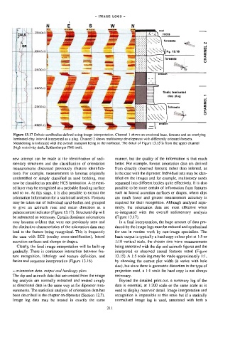
Figure 13.17 Deltaic sandbodies defined using image inlerpretation. Channel 1 shows an erosional base, foresets and an overlying
taminated clay interval interpreted as a plug. Channel 2 shows multistorey development with differently oriented foresets.
Meandering is indicated with the overall transport being to the northeast. The detail of Figure 13.15 is from the upper channel]
thigh resistivity dark, Schlumberger FMI too}).

new attempt can be made at the identification of sedi- manner, but the quality of the information is that much
mentary structures and the classification of orientation better. For example, foreset orientation data are derived
Measurements discussed previously (feature identifica- from directly observed foresets rather than inferred, as
tion). For example, measurements in Jaminae originally is the case with the dipmeter. Individual sets may be iden-
unidentified or simply classified as sand bedding, may tified on the images and for example, multistorey sands
now be classified as possible HCS tamination. A cement- separated into different bodies quite effectively. It is also
ed layer may be recognised as a probable flooding surface possible to be more certain of information from features
and so on. At this stage, it is also possible to extract the such as Jateral accretion surfaces or drapes, where dips
orientation information for a statistical analysis. Foresets are much lower and greater measurement accuracy is
may be taken out of individual sand-bodies and grouped required for their recognition. Although analysed sepa-
to give an azimuth rose and mean direction as a rately, the orientation data are most effective when
palaeocurrent indicator (Figure 13.17). Structural dip will re-integrated with the overall sedimentary analysis
be subtracted as necessary. Certain dominant orientations (Figure 13.17).
may become evident that were not previously seen and In a final interpretation, the huge amount of data pro-
the distinctive characteristics of the orientation data may duced by the image logs must be reduced and synthesised
lead to the feature being recognised. This is frequently for use in routine work by non-image specialists. The
the case with SCS (swaley cross-stratification), lateral basic output is typically a hard copy colour plot at 1:5 or
accretion surfaces and slumps or drapes. 1:10 vertical scale, the chosen sine wave measurements
Clearly, the final image interpretation wiil be built-up being annotated with the dip and azimuth figures and the
gradually. There is continuous interaction between fea- interpreted or observed causal features noted (Figure
ture recognition, lithology and texture definition, and 13.15). A 1:5 scale log may be made approximately 1:1.
facies and sequence interpretation (Figure 13.16). by choosing the correct plot width (it varies with hole
size), but since there is geometric distortion in the type of
- orientation data, output and hardcopy plots projection used, a 1:1] scale for hard copy is not always
The dip and azimuth data that are created from the image necessary.
fog analysis are normally extracted and treated simply Beyond the detailed print-out, a summary log of the
as directiona) data in the same way as for dipmeter mea- data is essential, at 1:200 scale or the same scale as is
surements. The statistical analysis of orientation data has used to display reservoir detail. Image interpretation and
been described in the chapter on dipmeter (Section 12.7). recognition is impossible at this scale but if a statically
Image log data may be treated in exactly the same normalised image log is used, annotated with both a

211