Page 222 - The Geological Interpretation of Well Logs

- THE GEOLOGICAL INTERPRETATION OF WELL LOGS —-

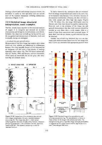
lithology column and a sedimentary structure coiumn, the To find a structural dip, orientation data are extracted
document is usable by non specialists and can include from the image interpretation and zoned in the same way
most of the features interpreted including sedimentary as for dipmeter data (Section 12,8). However. because of
orientation (Figure 3.17). the dominant sedimentary influence, the data will show a
very wide spread and ofien high dip angles (Figure
13.5 Electrical image structural 13.18). To reduce this, the image information must be
filtered: only shale dips should be used for structural dip.
interpretation, some examples
However, such is the accuracy of the image dip and
The first, simple, basic objective in the structural analysis azimuth measurement that thin shale sections should be
of images is to recognise and measure an accurate avoided as even these show a wide scatter, often as a
structural dip and recognise unconformities, even discon-
result of dips from concretions and cemented layers. If
formities. But objectives normally go far beyond this and thick shale intervals are chosen. a good structural dip can
the recognition and measurement of fractures, faults and be obtained.
eventually slumps are attempted. Another way of deriving structural dip is to use dip-
meter style measurements taken from the raw image tool
— structural dip and unconformities
data. Curves are selected in the appropriate posilion from
Measurement of dip from image logs tends to give values
which are very variable and influenced by sedimentary
features. Not every possible feature will be measured but
an interpreter wil] take quite a high density of readings
especially where values vary. This will favour sedimentary N E $ w N 8
dips (cf. Hurtey, 1994) and features such as concretions, thet =
a
2
which stand out electrically but do not give a the struc- 25
tural dip and azimuth values. = -
19th

A. IMAGE ANALYSIS — B. DIPMETER Wa £ 3
Be
o Oip > 90° O° Dip > 30° ° 3
a oo
2
2700 » SO Ex
ap ec
£ a
2
a
om €
¢
ao. °
' .

ergo a ‘eo 50d on
;
.
e [ate DILG | §
gee * B=
a5
mean
3 | Aye 50.8 || | 3 E
26
a
2e0a | - s ay
Be
€ 0, =
\ azimuth ‘ } = a 1 46
~4 ‘ dip z outer marine ™
/ histogram & shale
“i I y wf |
&
~ gk a
a» 4. u \ 1 lransgressive deposits
& re ws al |
3 * mse st a inesyattd ~~ arosional 60m
+t ww oo we om Mm fw 11° unconformity
2
a” Dip shallaw marina
R=333 N=200 sands

Figure 13.18 Comparison of the orientation data derived Figure 13.19 Electrica] image of an unconformily and
from image interpretation (A) and a standard dipmeter covering transgressive lag. The unconformily is seen as 4
processing (B). The image data show a wider spread sharp surface on the image with cementation below. The
reflecting greater detection of sedimentary features. Dipmeter uransgressive lag gives a speckled image although permeability
processing parameters: |.0m correlation interval, step 0.5m, is suggested by the colour (cored interval. high resistivity is
search angle 60°, The dipmeter processing is used for dark, Schlumberger FMI tool).
structural analysis.